Printing
  Demo 1
Cursor Icons
  Demo 2
MouseButtons
  Demo 3
PopupMenu
  Demo 4
Keystrokes
  Demo 5
Audio
  Demo 6
Timing & Speed
  Demo 7
Toolkit
  Demo 8
AppletContext
  Demo 9
Exercises

The JAIDA library is quite extensive and elaborate, so we cannot provide more than a brief introduction to it here. We will walk through the PolyFitJAIDAApp program displayed on the previous page and discuss the JAIDA code to provide a general idea as to how you can use it in your own code.

For more information, the JAIDA website offers resources like the API Documentation. The AIDA Manual describes both the Java and C++ versons of the libraries and can act as a general tutoral for the library. Other resources include a page on JAIDA Fit Methods and the Release Notes, which include a number of userful items such as a sample program showing how to add the JAIDA plotter to an application program. (We followed this approach in PolyFitJAIDAApp.) The AIDA Discussion Forum can help with questions you have about particular difficulties with the code.

In the PolyFitJAIDAApp program, several instance variables for JAIDA objects are listed at the top of the class description file. At the bottom of the file, the main() method creates an instance of the class, which is a JPanel subclass that will be added to a JFrame. The constructor invokes the init() method, which does the work of building the interface.

JAIDA Setup in init()

The init() method starts by creating several object factories:

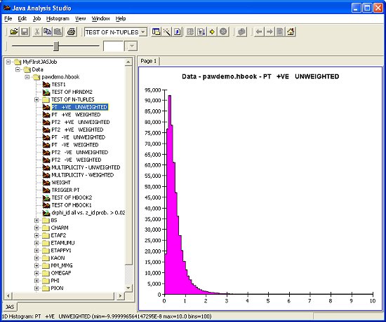
    // Create the JAIDA factory objects
    fAnalFactory           = IAnalysisFactory.create ();
    ITree tree             = fAnalFactory.createTreeFactory ().create ();
    fDpsFactory            = fAnalFactory.createDataPointSetFactory (tree);
    IHistogramFactory hf   = fAnalFactory.createHistogramFactory (tree);
    IFunctionFactory funcF = fAnalFactory.createFunctionFactory (tree);
    IFitFactory       fitF = fAnalFactory.createFitFactory ();

A factory refers to a static method that returns an instance of a class that you do not create directly with a constructor. This can be very convenient design pattern when there are setup parameters, such as those that vary with the platform, that are of no interest to the user of the object. The factory takes care of all the details of making the object and you simply start using the object after getting it from the factory.

The JAIDA framework relies completely on factories for creating objects. As shown by the JAIDA API, the library consists only of interfaces. So factories are the only way to instantiate objects that implement these interfaces.

The JAIDA software lets you organize your analysis data, plots, and histograms via a directory-style tree structure. Other than in the above factory object section, we don't take deal with the tree capability in the demo program here. However, it can be of great importance when handling the complexities of many different data sets and the histograms and plots for each. The JAS3 demo program shown here, for example,

displays the tree hierarchy of data and plots in the left frame of the program. The currently selected plot is displayed in the frame on the right.

So getting back to PolyFitJAIDAApp, we have created our factories and so in the next code lines,

    // Create a fitter
    fFitter  = fitF.createFitter ("Chi2","jminuit","noClone=true");
    fFitData = fitF.createFitData ();

we create an instance of the IFitter tool for doing our point and distribution fits. The arguments to the factory method tell it to use the JMinuit code for the fitting and to use the CHI2 minimization technique. (See the the Release Notes for a list of fitting techniques available in JMinuit.) The third argument is a technical detail that tells the fitter not to create an internal copy of of the fitted plot.

The IFitData object provides the data that the fitter will actually work on. It serves as an intermediate buffer that allows the fitter to work on a a standard data format regardless of the type of plot or histogram the data comes from.

Our own raw data points (the ones we will fit a polynomial to) must be placed into a IDataPointSet object for 2 dimensional data:

    // Create a two dimensional IDataPointSet.
    fDps2D = fDpsFactory.create ("dps2D","two dimensional IDataPointSet",2);

JAIDA allows for you to create a custom function to use for plotting and fitting:

    //Create a 1d second order polynomial
    fP2Func =
      funcF.createFunctionFromScript ("p2", 1, "a+b*x[0]+c*x[0]*x[0]",
                                      "a,b,c", "", null);

You will be able to access the three parameters of the polynomial via the names - a,b, and c. The function is named "p2".

JAIDA also provides some pre-defined functions such as the Gaussian:

    // Create Gaussian function for fitting residuals
    fGaussFunc = funcF.createFunctionByName("Gaussian", "G");

which we will use to fit our residuals distribution. To hold that we create a 1-D histogram:

    // Create fit residuals histogram
    fResidualsHist = hf.createHistogram1D ("Histogram 1D",50,-3,3);

The following code creates the plotting tool.

    // Create an IPlotter
    fPlotter = fAnalFactory.createPlotterFactory ().create ();
    // Create a region for the points plot and for the histogram.
    fPlotter.createRegions(2,1);

Here we use the createRegions() method to tell the plotter to create two areas where we will display the plot of points to fit and the residuals histogram.

The final JAIDA code in init() connects the plotter component to our the JPanel subclass PolyFitJAIDAApp, which in turn will be added to the JFrame instance:

    // Now embed the plotter into the application frame
    add (PlotterUtilities.componentForPlotter (fPlotter), BorderLayout.CENTER);

The other code in init() follows that in the original Chapter 8: Physics : LSQ Fit to a Polynominal program. It sets up the two text fields for input of the number of data points to fit and the sigma of the Gaussian smearing on the data points. It also adds buttons for initiating the plotting of the data, clearing the histogram, and ending the program.

Plotting, Histogramming and Fitting with JAIDA

When the user clicks on the "Go" button, the code in the actionPerformed() method will get the values from the text fields and then starts a thread. The class implements the Runnable interface and the run() method holds most of the code for carrying out the plot and fitting tasks.

The run() method holds a loop that runs over the number of plots requested in the first text field. The loop begins with an invocation of the genRanCurve() method that generates a quadratic polynomial with randomly selected parameters. Then "y" values at the given "x" positions are determined for this curve. For each point a Gauassian generated error factor is added to each point to emulate the smearing of real data with imprecise measurements. The sigma for that Gaussian is given by the value in the second text field. A random error bar is also created for each point.

The run() method loop then clears the IDataPointSet object and puts the x, y and y error bar values into it:

      // Clear the data point set
      fDps2D.clear ();

      // Fill the data point set with the generated data values.
      for (int j = 0; j < fX.length; j++ ) {
        fDps2D.addPoint ();
        fDps2D.point (j).coordinate (0).setValue (fX[j]);
        fDps2D.point (j).coordinate (1).setValue (fY[j]);
        fDps2D.point (j).coordinate (1).setErrorPlus (fYErr[j]);
      }

The data point set is connected to the fitter tool via the intermediate IFitData object:

      fFitData.create1DConnection (fDps2D,0,1);

The method arguments indicate that the first (0) dimension of the two-dimensional data set should be used as the x coordinate and the second dimension as the y coordinate in a fit of y=f(x).

The subsequent code deals with the fitting of the data. For some pathological cases, the fits may fail and throw run-time exceptions and stop the program. So we catch those exceptions. Two boolean variables

      boolean fit_p_ok = true;
      boolean fit_g_ok = true;

are used to flag whether an error condition has occurred.

The first fitting task is to fit a polynomial to the points that we generated:

        fFittedP = fFitter.fit (fFitData,fP2Func);

where fP2Func is the polynomial function object that we created in init().

We then obtain the parameters of the fitted function and calculate the residuals of the fit and fill the histogram:

        double [] fit_params = fFittedP.fittedParameters ();

        // Calculate the residual and fill the histogram
        for (int j=0; j < fX.length; j++) {
          double y_fit = fit_params[0] + fit_params[1]*fX[j]
                                  + fit_params[2]*fX[j]*fX[j];
          fResidualsHist.fill (fY[j] - y_fit);

The resulting distribution is then fit to a Gaussian

          fFittedG = fFitter.fit(fResidualsHist,fGaussFunc);

The following code clears the display areas and then plots the data points and overlays the fitted function in the first plot region. In the second region it plots the histogram and overlays it with the fitted Gaussian:

      // Clear the previous plot except for the very first time.
      if (!fFirstPlot) fPlotter.clearRegions ();
      fFirstPlot = false;

      // Plot and show the data with the fitted functions.
      fPlotter.region (0).plot (fDps2D);
      if (fit_p_ok) fPlotter.region(0).plot (fFittedP.fittedFunction () );
      fPlotter.region (1).plot (fResidualsHist);
      if (fit_g_ok) fPlotter.region(1).plot (fFittedG.fittedFunction () );
      fPlotter.show ();

Summary

The JAIDA code becomes fairly easy to follow once you understand the basic framework. It is quite powerful and you can quickly begin to take advantage of it for many different types of analysis work, not just for high energy physics.

There are many options and additional capabilities not dealt with here. See the documentation and examples on the JAIDA website for further exploration.

Most recent update: Dec.16, 2005

              Tech
Tech APIs
Exercises

           Physics
Math/Science APIs
JAIDA Program
  Demo 1
Demo 1 Discussion
Exercises