Java Tech - Chapter 12 : Physics

The JAIDA (and the corresponding C++ AIDA) library was developed in the High Energy Physics (HEP) community and parts of it, such as the HBOOK style histograms, can be traced back through two or three decades of program development at places like the CERN and SLAC accelerator facilities. For most of that time the programs were written in Fortran but now a pure Java version is available. (Until recently the Minuit fitting tools were still only available in native code but now the JMinuit.jar holds a Java version.) JAIDA is provided via the FreeHEP project.

As an example of using JAIDA classes with your own programs and n using a third-party physics analysis library in general, we created a program to carry out fits to data points with a polynomial. It is very similar to the program described in Chapter 8: Physics : LSQ Fit to a Polynominal but with the JAIDA tools for plotting and fitting.

Since there are a number of JAR files needed, we make the program just an application rather than an applet. To run PolyFitJAIDAApp, you will need to install the JAIDA packages on your system. Go to the java.freehep.org/jaida/ website and follow the instructions for downloading the JAIDA zip file and unpacking it into a convenient location.

To run the program from a command line, go to the JAIDA "bin" subdirectory and run the aida-setup command file appropriate for your platform. For example, on a Windows machine you would run aida-setup.bat as follows:

This command file will define the CLASSPATH environment variable so that the compiler and JVM will find the JAIDA packages. The second command adds the current directory to the classpath. The CLASSPATH variable will then go as :

(This would actually be one long line but line breaks were added here for clarity.)

After the above setup steps, move the command window to the directory with the program, e.g.

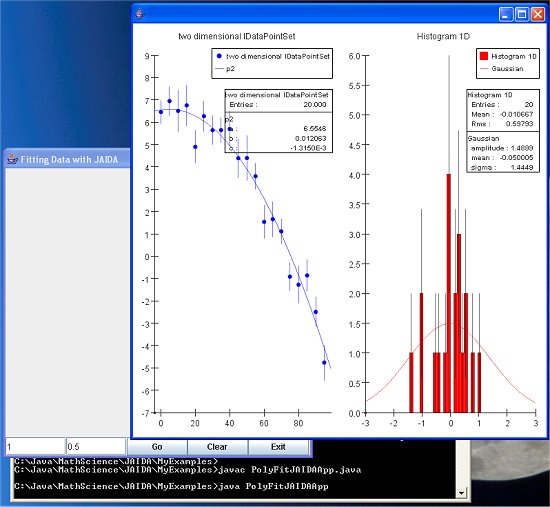
As shown in the image below, the program will open with the frame that holds similar text fields and buttons as the Chapter 8 program.. Clicking on "Go" will cause the JAIDA plotter frame to open and display the data points, a polynominal fitted through the points, a histogram showing a distribution of the residuals, and a Gaussian fit to the distribution. The results of the fit are shown in text boxes on each plot.

Clicking on "Go" repeatedly (or putting a larger number in the first data field and clicking once) will produced more fitted lines and the residuals histogram will gradually become more populated and the Gaussian fit will improve and eventually come to match well with the sigma value put in the second data field for the smearing of the data points. Hit "Clear" to clear the histogram and start over, e.g. with a new smearing sigma in the second text field.

Look over the code and then we will give a brief discussion of the JAIDA code used in the program.

PolyFitJAIDAApp

PolyFitJAIDAApp - Create data points in X vs Y and fit a polynominal to them. Use the JAIDA classes for the plotting and the fitting tasks.

import hep.aida.*;
import hep.aida.ref.plotter.PlotterUtilities;
import java.awt.*;
import java.awt.event.*;
import java.util.Random;
import javax.swing.*;

/**
  *
  *  This program combines PolyFitApplet with JAIDAEmbed
  *  to illustrate how to use JAIDA classes in your own
  *  GUI physics analysis program. Here we make it a pure
  *  app rather than an applet/app combo.
  *
  *  The program generates points along a quadratic curve and
  *  then fits a polynomial to them. This simulates typical
  *  physics analysis tasks such as fitting particle tracks
  *  through points provided by a wire detector.
  *
  *  The number of curves and the sigma of the smearing of the track
  *  measurement errors are taken from entries in two text fields.
  *  A  histogram holds the residuals
  *
  *  The "Go" button starts the track generation and fitting in a
  *  thread. "Clear"  button clears the histograms.
  *  In standalone mode, the Exit button closes the program.
  *
**/
public class PolyFitJAIDAApp extends JPanel
             implements ActionListener, Runnable
{

  // Define the various JAIDA instance variables
  IAnalysisFactory fAnalFactory;
  IDataPointSetFactory fDpsFactory;

  // The plotting tool.
  IPlotter fPlotter;

  // The data points to be plotted and fitted with a polynominal
  IDataPointSet fDps2D;

  // Functions for fitting the data points
  // and the residual distribution
  IFunction fP2Func;
  IFunction fGaussFunc;

  // Fitter variables
  IFitter fFitter;
  IFitData fFitData;
  IFitResult fFittedP;
  IFitResult fFittedG;

  // The histograms to record differences between
  // generated tracks and fitted tracks.
  IHistogram1D fResidualsHist;

  // Flag to indicate whether a plot has been made yet.
  boolean fFirstPlot = true;

  // Number of data plots to generate
  int fNumCurves = 1;

  // Scale of the data in x and y.
  double fYMin   =   0.0;
  double fYMax   =  10.0;
  double fXMin   =   0.0;
  double fXMax   = 100.0;

  // Arrays to hold data.
  double [] fX    = new double[20];
  double [] fY    = new double[20];
  double [] fYErr = new double[20];

  // Random number generator
  java.util.Random fRan;

  // Sigma to use for smearing of the points to fit.
  double fCurveSmear = 0.5;

  // Inputs for the number of tracks to generate
  JTextField fNumCurvesField;
  // and the smearing of the tracking points.
  JTextField fSmearField;

  //Buttons
  JButton fGoButton;
  JButton fClearButton;
  JButton fExitButton;

  // Use thread reference as flag.
  Thread fThread;

  /**  Creates a new instance of PolyFitJAIDAApp. The class
    *  extends JPanel. The main() method will create an
    *  instance of this class and add it to a JFrame.
   **/
  public PolyFitJAIDAApp () {
    super(new BorderLayout());
    // Build the GUI
    init ();

  } // ctor

  /**
    * Create a User Interface with histograms and buttons to
    * control the program. Two text files hold number of tracks
    * to be generated and the measurement smearing.
   **/
  public void init () {

    // Create the JAIDA factory objects
    fAnalFactory           = IAnalysisFactory.create ();
    ITree tree             = fAnalFactory.createTreeFactory ().create ();
    fDpsFactory            = fAnalFactory.createDataPointSetFactory (tree);
    IHistogramFactory hf   = fAnalFactory.createHistogramFactory (tree);
    IFunctionFactory funcF = fAnalFactory.createFunctionFactory (tree);
    IFitFactory       fitF = fAnalFactory.createFitFactory ();

    // Create a fitter
    fFitter  = fitF.createFitter ("Chi2","jminuit","noClone=true");
    fFitData = fitF.createFitData ();

    // Create a two dimensional IDataPointSet.
    fDps2D = fDpsFactory.create ("dps2D","two dimensional IDataPointSet",2);

    //Create a 1d second order polynomial
    fP2Func =
      funcF.createFunctionFromScript ("p2", 1, "a+b*x[0]+c*x[0]*x[0]",
                                      "a,b,c", "", null);

    // Create Gaussian function for fitting residuals
    fGaussFunc = funcF.createFunctionByName("Gaussian", "G");

    // Create fit residuals histogram
    fResidualsHist = hf.createHistogram1D ("Histogram 1D",50,-3,3);

    // Will need random number generator for generating tracks
    // and for smearing the measurement points
    fRan = new java.util.Random ();

    // Create an IPlotter
    fPlotter = fAnalFactory.createPlotterFactory ().create ();
    // Create a region for the points plot and for the histogram.
    fPlotter.createRegions(2,1);

    // Now embed the plotter into the application frame
    add (PlotterUtilities.componentForPlotter (fPlotter), BorderLayout.CENTER);

    // Use a textfield for an input parameter.
    fNumCurvesField =
      new JTextField (Integer.toString (fNumCurves), 10);

    // Use a textfield for an input parameter.
    fSmearField =
      new JTextField (Double.toString (fCurveSmear), 10);

    // If return hit after entering text, the
    // actionPerformed will be invoked.
    fNumCurvesField.addActionListener (this);
    fSmearField.addActionListener (this);

    fGoButton = new JButton ("Go");
    fGoButton.addActionListener (this);

    fClearButton = new JButton ("Clear");
    fClearButton.addActionListener (this);

    fExitButton = new JButton ("Exit");
    fExitButton.addActionListener (this);

    JPanel control_panel = new JPanel (new GridLayout (1,5));

    control_panel.add (fNumCurvesField);
    control_panel.add (fSmearField);
    control_panel.add (fGoButton);
    control_panel.add (fClearButton);
    control_panel.add (fExitButton);

    // Put control panel at bottom of panel.
    add (control_panel,"South");

    // Create dummy data to provide the x axis values
    // for the curves.
    double dx = 5.0;
    fX[0] = 0.0;
    for (int i=1; i < 20; i++){
        fX[i] = fX[i-1] + dx;
    }

  } // init

  /** Respond to controls. **/
  public void actionPerformed (ActionEvent e) {

    Object source = e.getSource ();
    if (source == fGoButton || source == fNumCurvesField
                           || source == fSmearField) {
      String strNumDataPoints = fNumCurvesField.getText ();
      String strCurveSmear = fSmearField.getText ();
      try{
          fNumCurves = Integer.parseInt (strNumDataPoints);
          fCurveSmear = Double.parseDouble (strCurveSmear);
      }
      catch (NumberFormatException ex) {
        // Could open an error dialog here but just
        // display a message on the browser status line.
        System.out.println ("Bad input value");
        return;
      }

      fGoButton.setEnabled (false);
      fClearButton.setEnabled (false);
      if (fThread != null) stop ();
      fThread = new Thread (this);
      fThread.start ();

    }
    else if ( source == fClearButton) {
        fResidualsHist.reset ();
        if (!fFirstPlot) fPlotter.clearRegions ();
        fFirstPlot = true;
    } else
        System.exit (0);

  } // actionPerformed

  public void stop (){
    // If thread is still running, setting this
    // flag will kill it.
    fThread = null;
  } // stop

  /**
    *  Generate the tracks in a thread and then
    *  fit the resulting points to a polynominal.
    *  Fill a histogram with the residuals and fit
    *  a Gaussian to it. This histogram will continue
    *  to fill until the Clear button is pushed.
   **/
  public void run () {

    for (int i=0; i < fNumCurves; i++){
      // Stop the thread if flag set
      if (fThread == null) return;

      // Generate a random track.
      double [] gen_params =
         genRanCurve (fXMax-fXMin,
                      fYMax-fYMin,
                      fX, fY, fYErr, fCurveSmear);

      // Clear the data point set
      fDps2D.clear ();

      // Fill the data point set with the generated data values.
      for (int j = 0; j < fX.length; j++ ) {
        fDps2D.addPoint ();
        fDps2D.point (j).coordinate (0).setValue (fX[j]);
        fDps2D.point (j).coordinate (1).setValue (fY[j]);
        fDps2D.point (j).coordinate (1).setErrorPlus (fYErr[j]);
      }

      // The data points are in a 2D data set. Use IFitData to tell
      // the fitter which coordinate (0) to treat as x and which to
      // treat as y (1) in a fit of y=f(x)
      fFitData.create1DConnection (fDps2D,0,1);
      boolean fit_p_ok = true;
      boolean fit_g_ok = true;

      // Fit a polynominal to the data points. In certain
      // pathological cases, the fit can fail to where an
      // exception is thrown. So we catch such exceptions
      // rather than letting the program stop.
      try {
        fFittedP = fFitter.fit (fFitData,fP2Func);
      }
      catch (Exception e) {
        System.out.println ("Fit exception: " + e);
        fit_p_ok = false;
      }

      // Residuals == difference between the measured value
      // and the fitted value at the points at each x position
      if (fit_p_ok) {
        // Get the parameters of the polymonial fit to the data.
        double [] fit_params = fFittedP.fittedParameters ();

        // Calculate the residual and fill the histogram
        for (int j=0; j < fX.length; j++) {
          double y_fit = fit_params[0] + fit_params[1]*fX[j]
                                  + fit_params[2]*fX[j]*fX[j];
          fResidualsHist.fill (fY[j] - y_fit);
        }
        // Now fit a Gaussian to the residuals distribution.
        // Catch exceptions if the fit fails.
        try {
          fFittedG = fFitter.fit(fResidualsHist,fGaussFunc);
        }
        catch (Exception e) {
          fit_g_ok = false;
          System.out.println ("Gaussian fit exception: " + e);
        }
      }

      // Clear the previous plot except for the very first time.
      if (!fFirstPlot) fPlotter.clearRegions ();
      fFirstPlot = false;

      // Plot and show the data with the fitted functions.
      fPlotter.region (0).plot (fDps2D);
      if (fit_p_ok) fPlotter.region(0).plot (fFittedP.fittedFunction () );
      fPlotter.region (1).plot (fResidualsHist);
      if (fit_g_ok) fPlotter.region(1).plot (fFittedG.fittedFunction () );
      fPlotter.show ();

      // Pause briefly to let users see the track.
      try {
          Thread.sleep (200);
      } catch (InterruptedException e) {}
    }

    fGoButton.setEnabled (true);
    fClearButton.setEnabled (true);

  } // run

  /**
    *  Generate a quadratic plot and obtain points along the curve.
    *  Smear the vertical coordinate with a Gaussian.
   **/
  double [] genRanCurve (double x_range, double y_range,
                         double [] x_curve, double [] y_curve,
                         double [] y_curve_err,
                         double smear){

    // Parameters for a quadratic line.
    double [] quadParam = new double[3];

    // Simulated quadratic
    double y0 = y_range* (0.5 + 0.25 * fRan.nextDouble ());
    double y1 = y_range * fRan.nextDouble ();

    // Choose some dummy paramters for the polynominal
    quadParam[0] = y0;
    quadParam[1] = (y1-y0)/ (8.0*x_range);
    quadParam[2] = (fRan.nextDouble () - 0.5)/100.0;

    // Make the points and errors along a quadratic line
    for (int i=0; i < x_curve.length; i++) {
      y_curve[i] = y0 + quadParam[1]*x_curve[i]
                     + quadParam[2]*x_curve[i]*x_curve[i];

      double curve_err = smear*fRan.nextGaussian ();

      // Add smear factor for this point
      y_curve[i] += curve_err;

      // Create a dummy average std.dev. error on the y value
      // for this x position.
      y_curve_err[i] =  (1.0 + fRan.nextDouble () ) * smear;

    }

    // Return the track parameters.
    return quadParam;

  } // genRanCurve

   /**
    * @param args the command line arguments
    */
   public static void main (String[] args) {
      int frame_width  = 450;
      int frame_height = 450;

      JFrame frame = new JFrame ("Fitting Data with JAIDA");
      frame.setDefaultCloseOperation (JFrame.EXIT_ON_CLOSE);

      frame.getContentPane ().add (new PolyFitJAIDAApp ());
      frame.setSize (new Dimension (frame_width,frame_height));
      frame.setVisible (true);

   } // main

} // PolyFitJAIDAApp